Triaxus
Geostatistical Analysis of TRIAXUS data
Client: Computer Science Corporation
Background
The Great Lakes National Program Office has been conducting regular surveillance monitoring of the offshore waters of the Great Lakes since 1983. This monitoring is intended to fulfill the provisions of the Great Lakes Water Quality Agreement calling for periodic monitoring of the lakes to: 1) assess compliance with jurisdictional control requirements; 2) provide information on non-achievement of agreed upon water quality objectives; 3) evaluate water quality trends over time; and 4) identify emerging problems in the Great Lakes basin ecosystem.
Assessing the condition of the nearshore presents substantial logistical challenges due to the large spatial extent involved and its characteristically high variability. Comprehensive monitoring of this region requires spatial resolution adequate to capture patterns and detect changes, something which would be prohibitively expensive and time consuming using traditional monitoring approaches. Assessment strategies employing in situ sensor technologies, on the other hand, offer the possibility of generating data at both a spatial scale and a level of resolution appropriate to characterizing highly variable and spatially extensive nearshore areas. This can be accomplished using a number of in situ sensors towed on a Triaxus instrument platform.
Objectives
The objective of the preliminary analysis of Triaxus data was two-fold:
- To visualize the spatial distribution of Lake Michigan nearshore data for a few key variables (conductivity, temperature and zooplankton density).
- To illustrate how geostatistics can help quantify and compare the spatial variability of these variables along the lateral and vertical directions.
Results
- The first objective was easily accomplished given the high spatial density of samples: 486,217 observations collected over the full length of the 769 km transect. No interpolation procedure was required and the observations were simply plotted using the public-domain Software SGeMS.
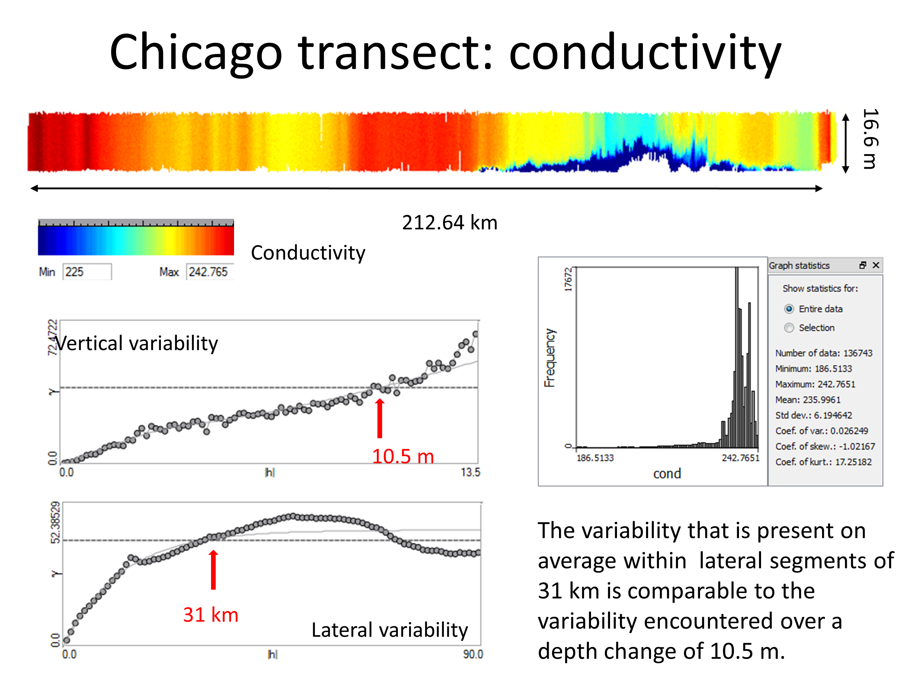
- The second objective required the computation of the variograms of each variable in the vertical and lateral directions. The variogram describes how the average squared difference between observations changes as a function of their separation distance. The analysis was accomplished using SpaceStat for two variables (conductivity, zooplankton density) and two transects: Chicago (136,735 observations for a length of 212.64 km) and Green Bay (47,651 observations for a length of 18.9 km) transects. The zooplankton data were first log-transformed to attenuate the impact of extreme values on the computation of the variogram. The comparison of the variability along the vertical and lateral directions was based on the distance at which the value of the vertical and lateral variograms exceeds the sample variance.